Network Creation

Setup

Import some useful Python packages to get started

# To create the networks
import metworkpy

# For performing some analysis of the networks
import networkx as nx

# For network visualization
import iplotx as ipx
import matplotlib.pyplot as plt

# For handling the Models
import cobra

Configure COBRApy to use the glpk solver since it comes with that automatically, and it will be fast enough for this tutorial

cobra.Configuration().solver = "glpk"

Get an Example COBRA Model

MetworkPy includes a simple example COBRApy Model which we will use for this tutorial

model = metworkpy.examples.get_example_model()

Create a Metabolic Network

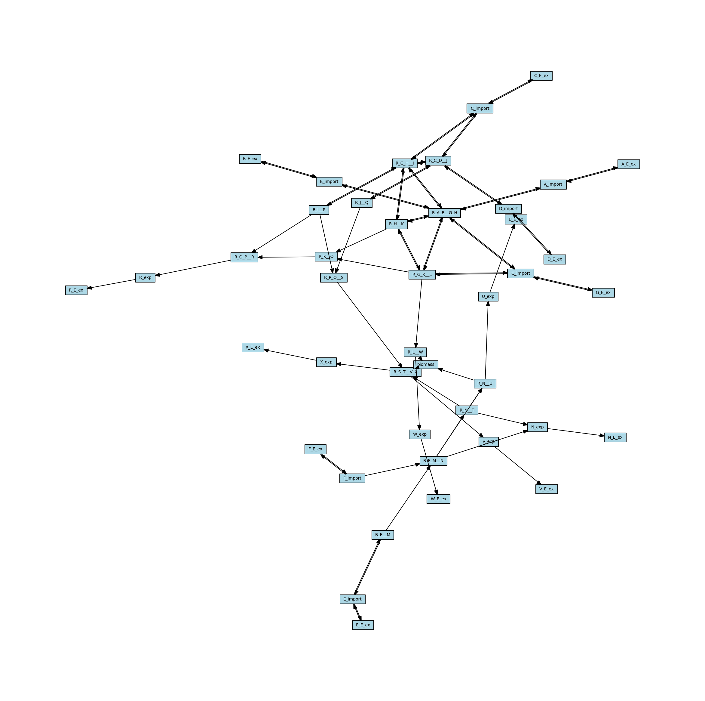
MetworkPy enables the creation of several different kinds of networks from the COBRApy Model, we will start with the stoichiometric connectivity networks, specifically the bipartite metabolic network. This network represents connections between the metabolites and reactions in the COBRApy Model based on which reactions act on which metabolites. The network includes nodes for all of the metabolites and reactions in the model. Edges connect metabolite nodes to reaction nodes (and vis-versa) if the metabolite is a substrate of a reaction. These networks can be optionally directed and weighted, but for now we will stick to the simplest version.

# Create the metabolic network
metabolic_network = metworkpy.create_metabolic_network(
    model=model,  # The input COBRApy model to create the network from
    weighted=False,  # Don't add weights to the network
    directed=False,  # Create an undirected network
)

# Check that the returned network is a NetworkX Graph
assert isinstance(metabolic_network, nx.Graph), (
    "Oh No! Something has gone terribly wrong!"
)

We can use iplotx and Matplotlib to visualize this network we have created:

# Create a list of metabolites and reactions so that they can be colored differently
reaction_list = [r.id for r in model.reactions]
metabolite_list = [m.id for m in model.metabolites]

# Create the matplotlib Figure and Axes to show the network
fig, ax = plt.subplots()
fig.set_size_inches(
    30, 30
)  # Increase the figure size so the nodes are more readable

# Create a list of node colors
reaction_color = "lightblue"  # Color for reaction nodes
metabolite_color = "red"  # Color for metabolite nodes
node_color_list = []  # List of node colors in order that the network is traversed
for node in metabolic_network.nodes:
    if node in reaction_list:
        node_color_list.append(reaction_color)
    elif node in metabolite_list:
        node_color_list.append(metabolite_color)

# Plot the network
ipx.network(
    metabolic_network,  # The network to visualize
    ax=ax,  # The matplotlib axes to draw on
    layout=nx.spring_layout(
        metabolic_network, seed=314
    ),  # Layout to use, using NetworkX's spring layout
    vertex_marker="r",  # Draw the nodes as rectangles
    vertex_labels=True,  # Add a label to the nodes
    vertex_facecolor=node_color_list,  # Set the colors of the nodes
    style="hollow",  # Allow the labels to be seen
)

[<iplotx.network.NetworkArtist at 0x7fd1553ba750>]

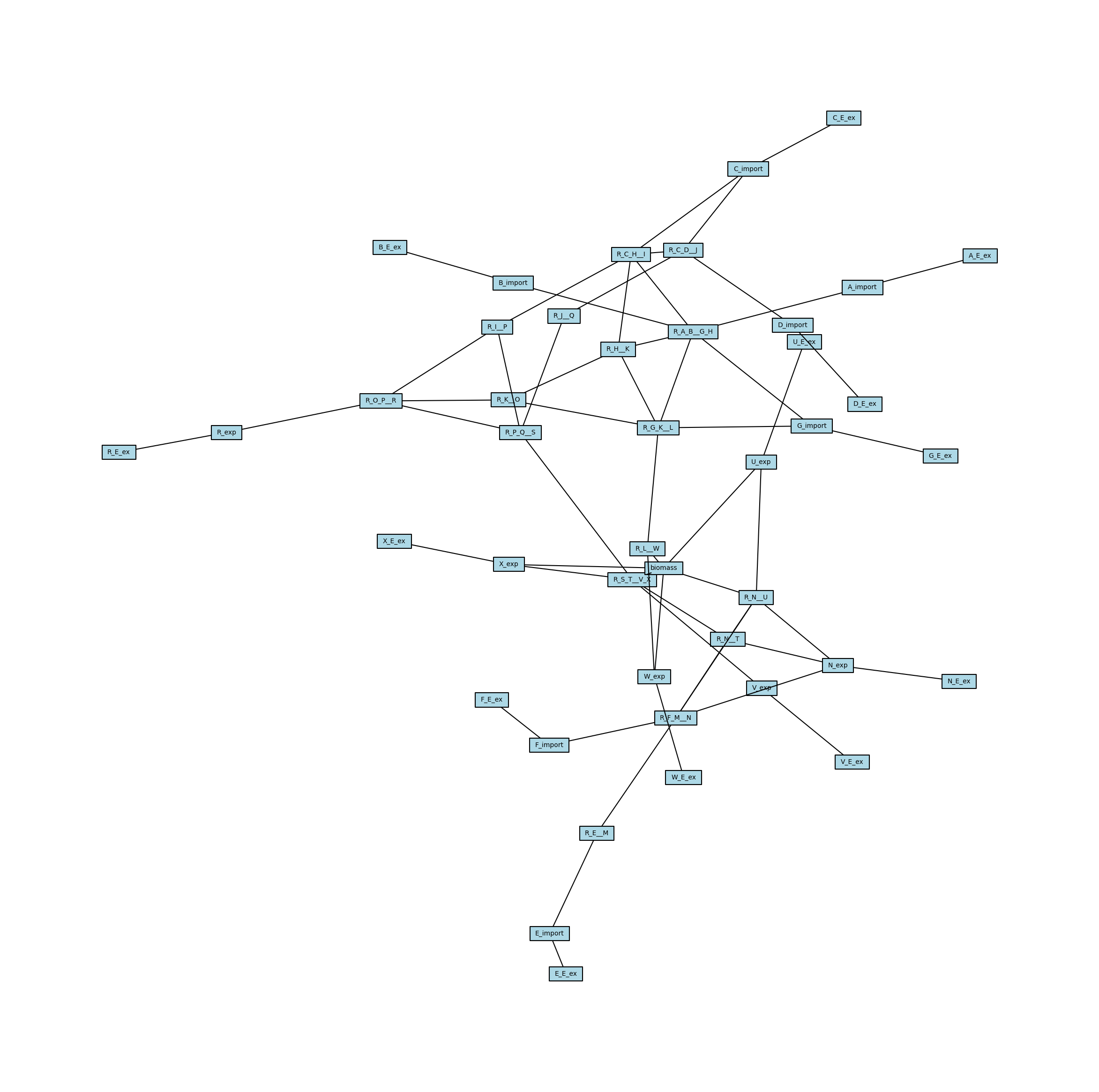
Create a Reaction Network

Sometimes it is more useful to be able to analyze the connectivity of only reactions (or only metabolites, see below). To do this, we can project the above Bipartite network (meaning that all of the edges go between two groups of nodes, in this case reaction nodes and metabolite nodes) onto a subset of nodes. This is done by creating a new network with only a subset of nodes (specifically one of the two node sets in the bipartite network), and connecting them if they share a neighbor in the other node set. In the case of the reaction connectivity network, this means that the reactions are connected if they both share a metabolite as a substrate.

# Create the network of reactions only
reaction_network = metworkpy.bipartite_project(
    metabolic_network,
    node_set=model.reactions.list_attr(
        "id"
    ),  # This is a way of getting the reaction IDs from the COBRApy Model
)

MetworkPy also contains a helper function to create this reaction connectivity network directly:

reaction_network = metworkpy.create_reaction_network(
    model=model, weighted=False, directed=False
)

We can then visualize this reaction connectivity network, plotting it with the same layout at the bipartite metabolic network so they can be easily compared

# Create the matplotlib Figure and Axes to show the network
fig, ax = plt.subplots()
fig.set_size_inches(
    30, 30
)  # Increase the figure size so the nodes are more readable

# Plot the network
ipx.network(
    reaction_network,  # The network to visualize
    ax=ax,  # The matplotlib axes to draw on
    # Use the layout of the full network so that they can be easily compared
    layout=nx.spring_layout(
        metabolic_network, seed=314
    ),  # Layout to use, using NetworkX's spring layout
    vertex_marker="r",  # Draw the nodes as rectangles
    vertex_labels=True,  # Add a label to the nodes
    vertex_facecolor="lightblue",  # Set the colors of the nodes
    style="hollow",  # Allow the labels to be seen
)

[<iplotx.network.NetworkArtist at 0x7fd1a41b2240>]

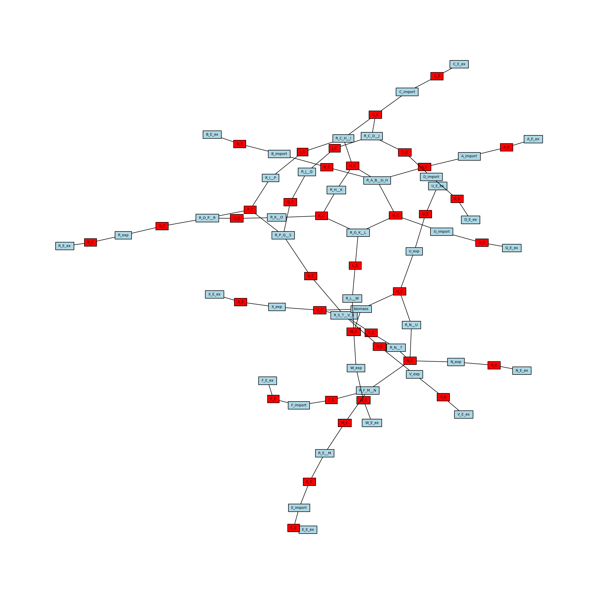
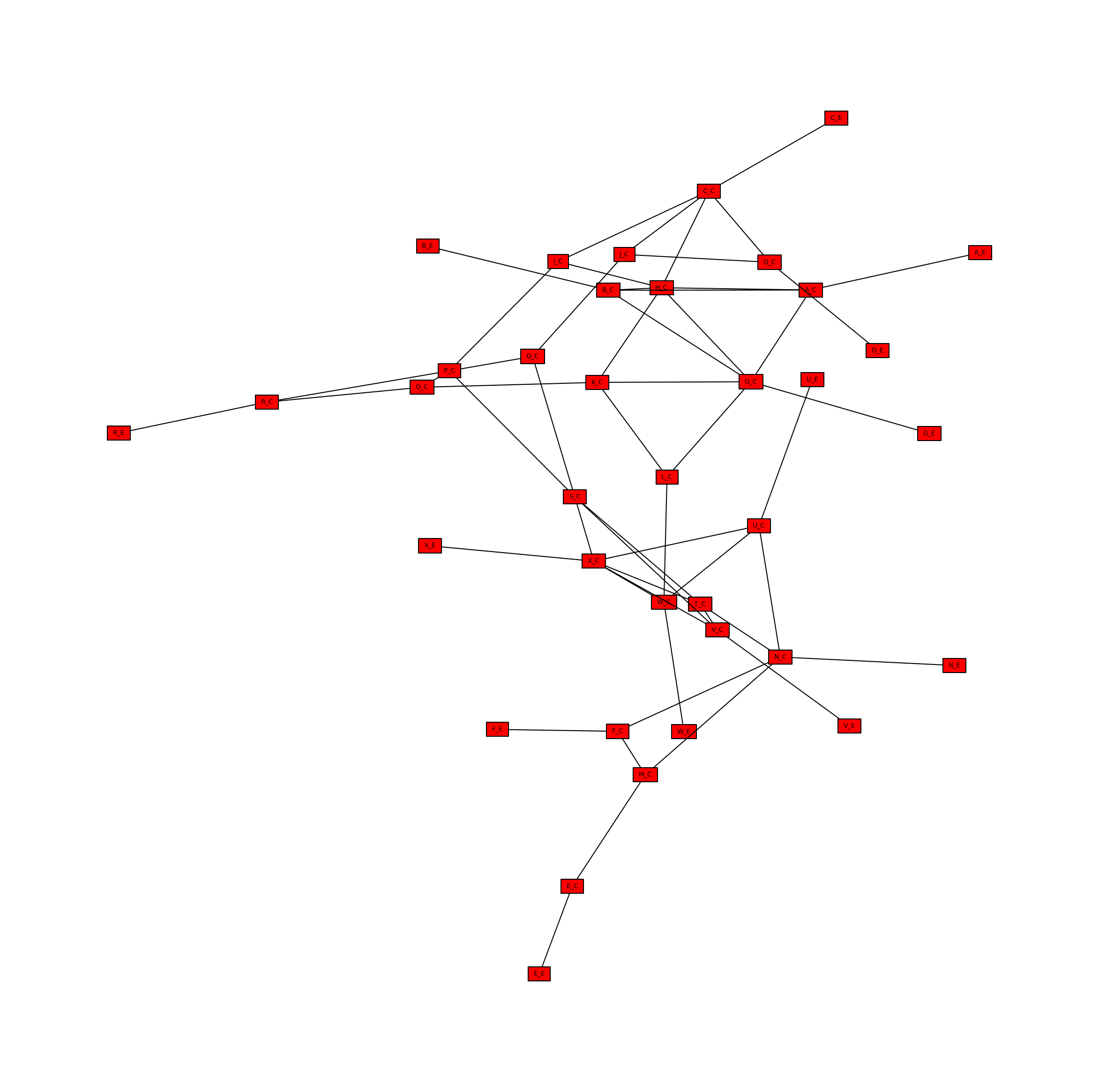
Create a Metabolite Network

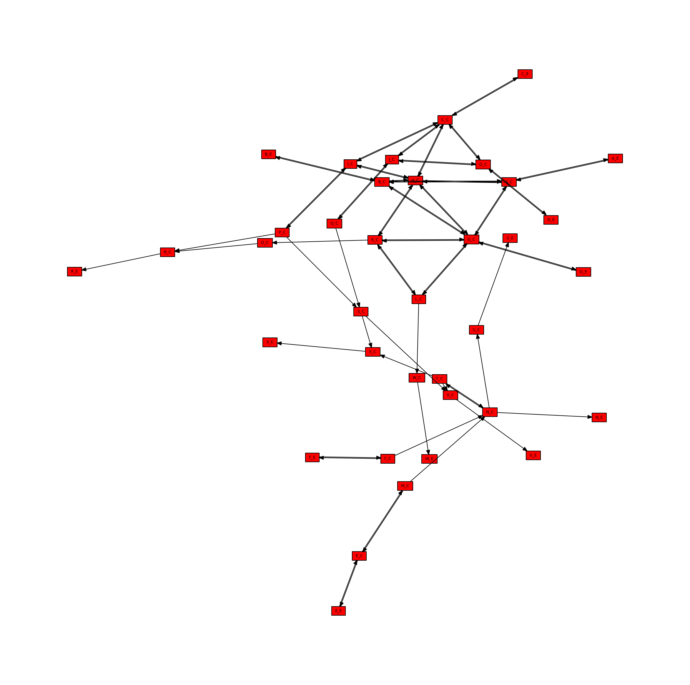
In a simmilar way, the bipartite metabolic network can be projected onto only the metabolite nodes. This time, metabolite nodes are connected if they are the substrate of the same reaction. We will use another helper function to create this network directly, rather than projecting the bipartite metabolic network, but the two methods are equivalent.

metabolite_network = metworkpy.create_metabolite_network(
    model=model, weighted=False, directed=False
)

We can then visualize this network

# Create the matplotlib Figure and Axes to show the network
fig, ax = plt.subplots()
fig.set_size_inches(
    30, 30
)  # Increase the figure size so the nodes are more readable

# Plot the network
ipx.network(
    metabolite_network,  # The network to visualize
    ax=ax,  # The matplotlib axes to draw on
    # Use the layout of the full network so that they can be easily compared
    layout=nx.spring_layout(
        metabolic_network, seed=314
    ),  # Layout to use, using NetworkX's spring layout
    vertex_marker="r",  # Draw the nodes as rectangles
    vertex_labels=True,  # Add a label to the nodes
    vertex_facecolor="red",  # Set the colors of the nodes
    style="hollow",  # Allow the labels to be seen
)

[<iplotx.network.NetworkArtist at 0x7fd155521820>]

Directed Network

Directed Metabolic Network

The stoichiometric connectivity networks can also be directed. This means that the edges in the network will have an orientation, so they will go from one node to another instead of just connecting two nodes. The direction is intended to reflect the direction that metabolites can move through the network, so an edge connecting a metabolite to a reaction indicates that the reaction can consume that metabolite, whereas an edge from a reaction to a metabolite indicates that the reaction can generate that metabolite. Here is the directed version of the metabolic network, with arrows representing the directionality of the edges.

# Create the directed metabolic network
metabolic_network_directed = metworkpy.create_metabolic_network(
    model=model, directed=True, weighted=False
)


# Visualize this network
# Create the matplotlib Figure and Axes to show the network
fig, ax = plt.subplots()
fig.set_size_inches(
    30, 30
)  # Increase the figure size so the nodes are more readable

# Create a list of node colors
reaction_color = "lightblue"  # Color for reaction nodes
metabolite_color = "red"  # Color for metabolite nodes
node_color_list = []  # List of node colors in order that the network is traversed
for node in metabolic_network.nodes:
    if node in reaction_list:
        node_color_list.append(reaction_color)
    elif node in metabolite_list:
        node_color_list.append(metabolite_color)

# Plot the network
ipx.network(
    metabolic_network_directed,  # The network to visualize
    ax=ax,  # The matplotlib axes to draw on
    # Use the layout of the full network so that they can be easily compared
    # Using the layout for the undirected network for consistency
    layout=nx.spring_layout(metabolic_network, seed=314),
    vertex_marker="r",  # Draw the nodes as rectangles
    vertex_labels=True,  # Add a label to the nodes
    vertex_facecolor=node_color_list,  # Set the colors of the nodes
    style="hollow",  # Allow the labels to be seen
)

[<iplotx.network.NetworkArtist at 0x7fd155492cc0>]

Directed Reaction Network

This directed bipartite metabolic network can also be projected onto node subsets, for example the set of reactions. In this projection reaction nodes will be connected in the direction of a path between them in bipartite network. That is, if you have two nodes A and B, there will be an edge from A to B if there is a directed path (a path moving along the directed edges) from A to B. Simmilarly, there will be an edge from B to A if there is a directed path from B to A. Below is an example of projecting the bipartite metabolite network onto the reaction nodes.

reaction_network_directed = metworkpy.create_reaction_network(
    model=model, directed=True, weighted=False
)

# Create the matplotlib Figure and Axes to show the network
fig, ax = plt.subplots()
fig.set_size_inches(
    30, 30
)  # Increase the figure size so the nodes are more readable

# Plot the network
ipx.network(
    reaction_network_directed,  # The network to visualize
    ax=ax,  # The matplotlib axes to draw on
    # Use the layout of the full network so that they can be easily compared
    layout=nx.spring_layout(
        metabolic_network, seed=314
    ),  # Layout to use, using NetworkX's spring layout
    vertex_marker="r",  # Draw the nodes as rectangles
    vertex_labels=True,  # Add a label to the nodes
    vertex_facecolor="lightblue",  # Set the colors of the nodes
    style="hollow",  # Allow the labels to be seen
)

[<iplotx.network.NetworkArtist at 0x7fd154680740>]

Directed Metabolite Network

The network can simmilarly be projected onto only the metabolite nodes, visualized below.

# Create the directed metabolite network
metabolite_network_directed = metworkpy.create_metabolite_network(
    model=model, directed=True, weighted=False
)

# Create the matplotlib Figure and Axes to show the network
fig, ax = plt.subplots()
fig.set_size_inches(
    30, 30
)  # Increase the figure size so the nodes are more readable

# Plot the network
ipx.network(
    metabolite_network_directed,  # The network to visualize
    ax=ax,  # The matplotlib axes to draw on
    # Use the layout of the full network so that they can be easily compared
    layout=nx.spring_layout(
        metabolic_network, seed=314
    ),  # Layout to use, using NetworkX's spring layout
    vertex_marker="r",  # Draw the nodes as rectangles
    vertex_labels=True,  # Add a label to the nodes
    vertex_facecolor="red",  # Set the colors of the nodes
    style="hollow",  # Allow the labels to be seen
)

[<iplotx.network.NetworkArtist at 0x7fd1546788c0>]

Weighted Network

The networks can also have weighted edges. MetworkPy currently allows for two weighting methods, either by stoichiometric coefficient, or by flux. Since the example network has only unit stoichiometric coefficients, we will look at the flux based approach. This method first finds the maximum and minimum flux that can flow through a reaction using the `flux_variability_analysis <https://cobrapy.readthedocs.io/en/latest/autoapi/cobra/flux_analysis/variability/index.html>`__ method of COBRApy, and uses this to identify the amount of metabolite flux that can flow from metabolites to reactions, and from reactions to metabolites. Note that the fluxes found with the flux_variability_analysis are the maximum/minimum fluxes while still optimizing the objective function. This can be changed by changing the model objective function prior to passing it to the create_metabolic_network function, or by setting the kwarg fraction_of_optimum to a lower value (potentially 0.0).

For edges in this network, there are several cases to consider:

• Edges from metabolites to reactions represent the maximum flux of a metabolite that can be consumed by the reaction

  • The metabolite is a reactant of the reaction: The weight is the maximum positive flux of the reaction, multiplied by the stoichiometric coefficient of the metabolite in the reaction. If the reaction can only act in reverse, this value is 0.

  • The metabolite is a product of the reaction: The weight is the maximum negative flux of the reaction, multiplied by the stoichiometric coefficient of the metabolite in the reaction. If the reaction can only act in the forward direction, this value is 0. Note that the value of this weight is still positive, and that the negative sign is captured by the directionality of the edge (since it is from a product of the reaction towards the reaction).

• Edges from reactions to metabolites represent the maximum flux of a metabolite that can be generated by the reaction

  • The metabolite is a reactant of the reaction: The weight is the maximum negative flux of the reaction, multiplied by the stoichiometric coefficient of the metabolite in the reaction. If the reaction can only act in the forward direction, this value is 0. Note that the weight is still positive, with the negative sign being captured by the directionality of the edge (since it is from a reaction to its reactant).

  • The metabolite is a product of the reaction: The weight is the maximum positive flux of the reaction, multiplied by the stoichiometric coefficient of the metabolite in the reaction. If the reaction can only act in reverse, this value is 0. Below is an example of a weighted and directed network.

# Create the directed metabolic network
metabolic_network_weighted = metworkpy.create_metabolic_network(
    model=model,
    directed=True,
    weighted=True,
    weight_by="fva",
    # We can pass additional keyword arguments in,
    # which will be passed to the flux_variability_analysis method of COBRApy
    # For example the fraction_of_optimum can be set to control how close to
    # optimal biomass production the model has to stay while finding the
    # maximum and minimum flux for each reaction
    fraction_of_optimum=0.1,
    # The fraction of optimum can also be set to 0.0, which will mean
    # that the flux values are just the maximum
)


# Visualize this network
# Create the matplotlib Figure and Axes to show the network
fig, ax = plt.subplots()
fig.set_size_inches(
    30, 30
)  # Increase the figure size so the nodes are more readable

# Create a list of node colors
reaction_color = "lightblue"  # Color for reaction nodes
metabolite_color = "red"  # Color for metabolite nodes
node_color_list = []  # List of node colors in order that the network is traversed
for node in metabolic_network.nodes:
    if node in reaction_list:
        node_color_list.append(reaction_color)
    elif node in metabolite_list:
        node_color_list.append(metabolite_color)

# Create a dict of the edge widths
# Scale the edges so that they can actually be visualized
scale_factor = 0.25
metabolic_network_weighted_edge_widths = {
    (u, v): w["weight"] * scale_factor
    for (u, v, w) in metabolic_network_weighted.edges(data=True)
}

# Plot the network
ipx.network(
    metabolic_network_weighted,  # The network to visualize
    ax=ax,  # The matplotlib axes to draw on
    # Use the layout of the full network so that they can be easily compared
    # Using the layout for the undirected network for consistency
    layout=nx.spring_layout(metabolic_network, seed=314),
    vertex_marker="r",  # Draw the nodes as rectangles
    vertex_labels=True,  # Add a label to the nodes
    vertex_facecolor=node_color_list,  # Set the colors of the nodes
    edge_linewidth=metabolic_network_weighted_edge_widths,  # Set the width of the edges based on the edge weights
    style="hollow",  # Allow the labels to be seen
)

[<iplotx.network.NetworkArtist at 0x7fd15461b680>]

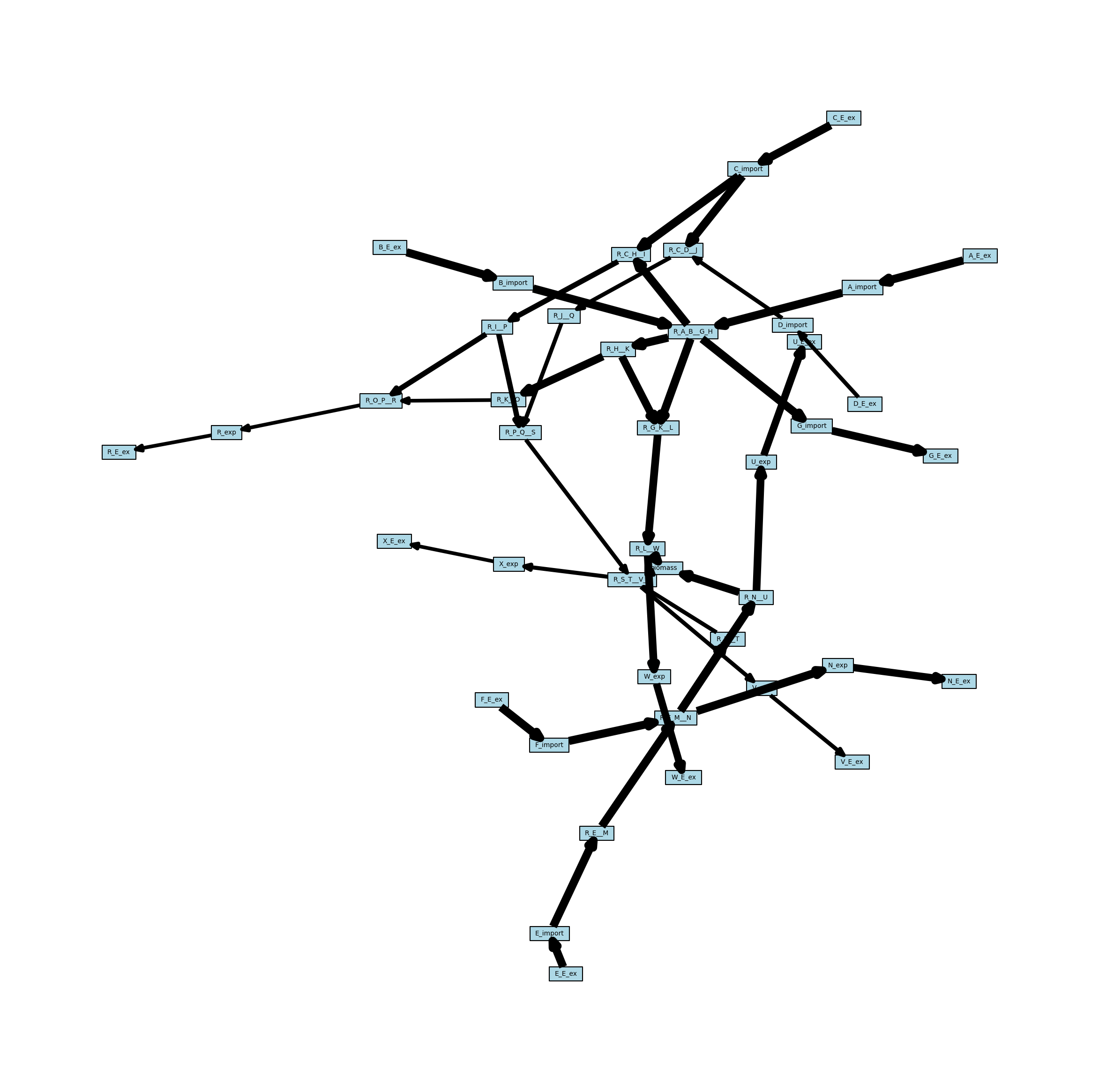
Weighted Reaction Network

This weighted network can also be projected onto the reaction nodes, but required some additional consideration for how weights are handled. When projecting onto reactions, the edges in the new network are essentially combining two other edges (one from reaction 1 to a metabolite, and one from the metabolite to reaction 2). MetworkPy allows for selecting the method to do this by passing a callable (function or class with a __call__ method) to the bipartite project function. Here, we will just use the default, which is the maximum.

reaction_network_weighted = metworkpy.create_reaction_network(
    model=model,
    directed=True,
    weighted=True,
    weight_by="fva",
    fraction_of_optimum=0.1,
)

# Create the matplotlib Figure and Axes to show the network
fig, ax = plt.subplots()
fig.set_size_inches(
    30, 30
)  # Increase the figure size so the nodes are more readable

# Create a dict of the edge widths
# Scale the edges so that they can actually be visualized
scale_factor = 0.25
reaction_network_weighted_edge_widths = {
    (u, v): w["weight"] * scale_factor
    for (u, v, w) in reaction_network_weighted.edges(data=True)
}

# Plot the network
ipx.network(
    reaction_network_weighted,  # The network to visualize
    ax=ax,  # The matplotlib axes to draw on
    # Use the layout of the full network so that they can be easily compared
    layout=nx.spring_layout(
        metabolic_network, seed=314
    ),  # Layout to use, using NetworkX's spring layout
    vertex_marker="r",  # Draw the nodes as rectangles
    vertex_labels=True,  # Add a label to the nodes
    vertex_facecolor="lightblue",  # Set the colors of the nodes
    edge_linewidth=reaction_network_weighted_edge_widths,  # Set the width of the edges based on the edge weights
    style="hollow",  # Allow the labels to be seen
)

[<iplotx.network.NetworkArtist at 0x7fd1557629f0>]

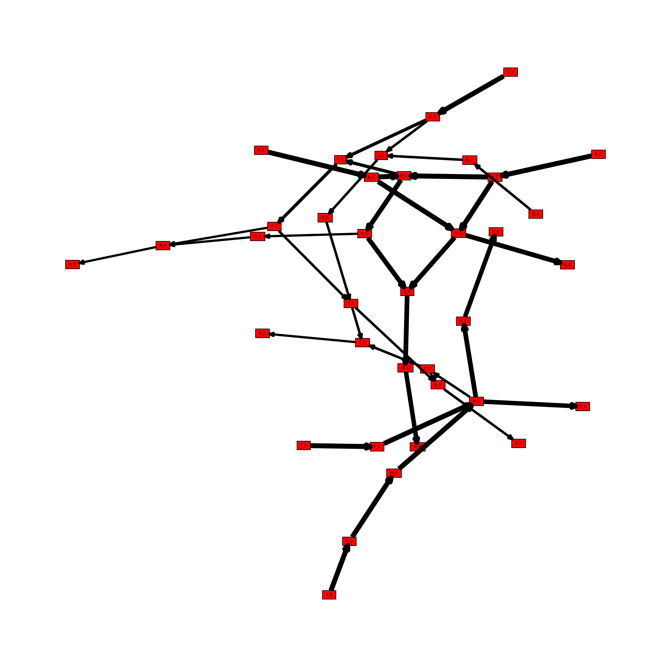
Weighted Metabolite Network

The network can also be projected onto only the metabolites in a simmilar manner. See an example below.

# Create the directed metabolite network
metabolite_network_weighted = metworkpy.create_metabolite_network(
    model=model,
    directed=True,
    weighted=True,
    weight_by="fva",
    fraction_of_optimum=0.1,
)

# Create the matplotlib Figure and Axes to show the network
fig, ax = plt.subplots()
fig.set_size_inches(
    30, 30
)  # Increase the figure size so the nodes are more readable

# Create a dict of the edge widths
# Scale the edges so that they can actually be visualized
scale_factor = 0.25
metabolite_network_weighted_edge_widths = {
    (u, v): w["weight"] * scale_factor
    for (u, v, w) in metabolite_network_weighted.edges(data=True)
}

# Plot the network
ipx.network(
    metabolite_network_weighted,  # The network to visualize
    ax=ax,  # The matplotlib axes to draw on
    # Use the layout of the full network so that they can be easily compared
    layout=nx.spring_layout(
        metabolic_network, seed=314
    ),  # Layout to use, using NetworkX's spring layout
    vertex_marker="r",  # Draw the nodes as rectangles
    vertex_labels=True,  # Add a label to the nodes
    vertex_facecolor="red",  # Set the colors of the nodes
    edge_linewidth=metabolite_network_weighted_edge_widths,  # Set the width of the edges based on the edge weights
    style="hollow",  # Allow the labels to be seen
)

[<iplotx.network.NetworkArtist at 0x7fd154360b90>]

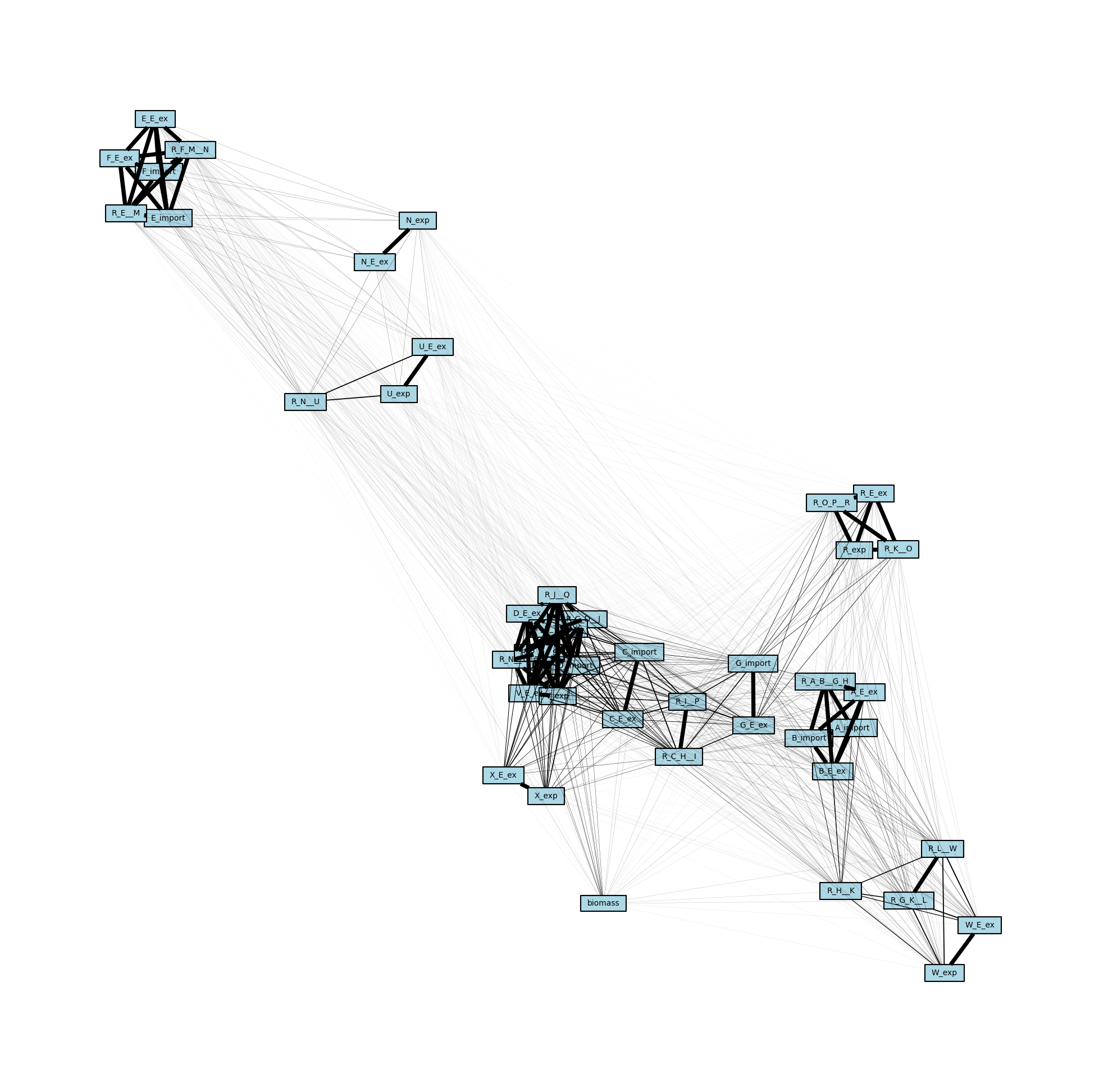
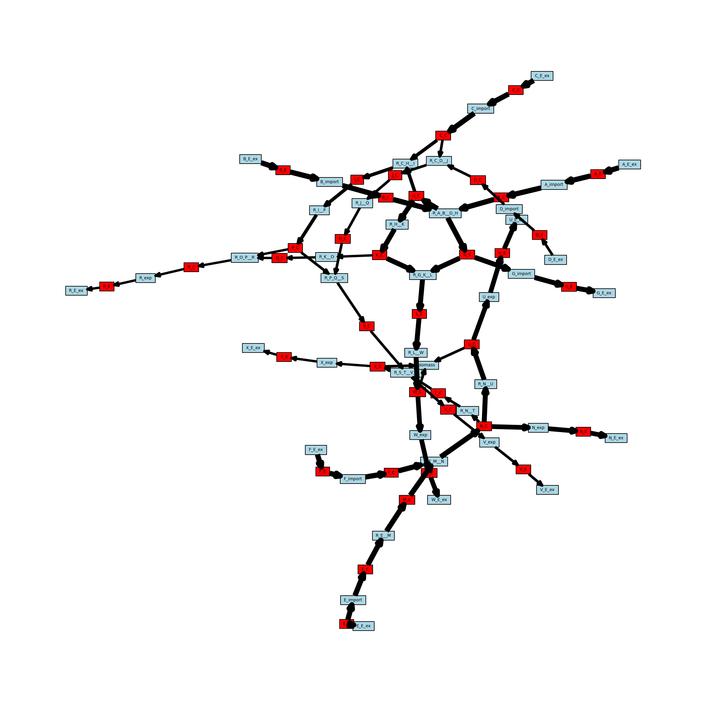
Create a Mutual Information Network

In addition to the stoichiometric connectivity networks above, MetworkPy can also create a flux mutual information network. This network includes nodes for all of the reactions in the model, and uses the mutual information between the flux of these reactions to weight the edges between them. Mutual information is a measure of statistical dependence that is sensitive to the relationships between the means, the variances, or the higher moments of two distributions.

Given two related random variables, mutual information captures how much information is gained about one variable given that we know the value of the other. In the case of the flux mutual information network then, the edge weights indicate how much information is gained about the flux state of the reaction at one end of the edge given knowledge of the flux state of the reaction at the other end of the edge. This is generally higher for reactions that are closer together, but can reveal information about more distant relationships as well. For example, if there are two paths through a particular part of the metabolism, then knowing the flux state of reactions on one side of those parallel paths gives a significant amount of information about the state of reactions on the other path (if the flux through one side is very high, it indicates it is taking up a significant portion of upstream production, and so the flux on the other side is likely to be lower).

flux_mi_network = metworkpy.create_mutual_information_network(
    model=model, n_samples=1_000, processes=1
)

We can again visualize this network using iplotx, which reveals several node clusters.

# Create a dict from edge to weight
mi_edge_widths = {
    (u, v): w["weight"] for (u, v, w) in flux_mi_network.edges(data=True)
}

fig, ax = plt.subplots()
fig.set_size_inches(25, 25)

ipx.network(
    flux_mi_network,
    ax=ax,
    layout=nx.spring_layout(flux_mi_network, seed=1892382),
    vertex_marker="r",
    vertex_labels=True,
    vertex_facecolor="lightblue",
    style="hollow",
    edge_linewidth=mi_edge_widths,
)

[<iplotx.network.NetworkArtist at 0x7fd1545c2780>]